Fingerprints of ‘natural’ climate variability.

1. The Great Climate Shift. Something of a mystery. We can certainly say what happened, but can we say what caused what, and how?
   
2. Combined solar cycles (red) correlate with temperatures: 1000frolly
   
3. Sea level follows the sun:
   
4. Data from all reporting agencies agree that at least as far back as 2002 average global temperature tracks water vapor, not CO2 (Figure 0.2). Hat-tip: Dan Pangburn.
   
5. Atlantic ocean cycles, AMO, and land surface temperature in the Eastern USA show delayed correlation:

6. Correlations of global sea surface temperatures with the solar wind speed:
   https://www.sciencedirect.com/science/article/pii/S1364682616300360

   They concluded: Responses of sea-surface temperature to solar wind speed on the seasonal timescale have been found, and in the North Atlantic region in winter they resemble the North Atlantic Oscillation. At the locations of the peak (negative) response in the North Atlantic the SST decreases by approximately 1°C for 100 km s^-1 increase in solar wind speed. In the southern hemisphere regions of significant positive and negative correlations with SWS are smaller and less well organized. The analysis is made for 1963-2010 data, and the effect strongest in winter, and greater when the solar wind magnetic field is southward, ensuring greater energy input into the ionosphere-atmosphere system. The response is somewhat stronger in the west phase of the QBO than in the east phase, and stronger than when F10.7 is used for the correlations. These seasonal responses are consistent with cumulative effects of a prompt electrical mechanism affecting cloud microphysics, as found elsewhere. However, on the seasonal timescale there is ambiguity as to which of several inputs to the stratosphere or troposphere is driving the responses. It is even possible that upward propagating waves, resulting from short term responses to the solar wind, are changing the strengths of the northern and southern polar vortices, which on longer timescales cause downward propagating dynamical disturbances that affect the NAO and the southern oceans.

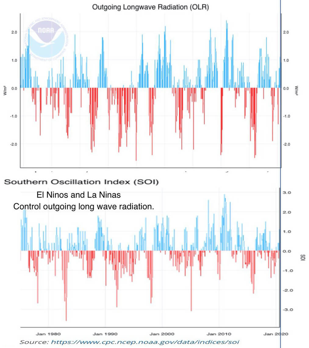
7. Over the pacific: Outgoing longwave radiation to space correlates with ocean cycles:
   

8. Solar cycles significantly affect seismic activity.
   
   Volvanoes and earthquakes happen at seismic fault lines where tectonic plates overlap.

   "In this paper, we analyze 20 years of proton density and velocity data, as recorded by the SOHO satellite, and the worldwide seismicity in the corresponding period, as reported by the ISC-GEM catalogue. We found clear correlation between proton density and the occurrence of large earthquakes (M> 5.6), with a time shift of one day. The signifcance of such correlation is very high, with with probability to be wrong lower than 10^-5 " [meaning one in 10000] ... In this paper, we demonstrate that it [the correlation] can likely be due to the effect of solar wind, modulating the proton density and hence the electrical potential between the ionosphere and the Earth ... our hypothesis only implies that the proton density would act as a further, small trigger to cause the fracture on already critically charged faults, thus producing the observed large scale earthquake correlation."

   Marchitelli et al only claim an fingerprint between seismicity and solar wind proton density. Increased seismicity leads to both volcanos and earthquakes. Only earthquakes were used in the data because there are tens of thousands per year; leading to excellent statistical certainty. in contrast there are about 25+ new volcanoes each year; too few to give good statistical certainty.

   Links: Salon | Nature (paper, open access)

9. 
10. 
11. Precipitation vs. Sunspot numbers. February precipitation in Germany compared to changes in sunspots. Shown is the optimum positive correlation (r = 0.54) with a solar lag of +17 months. Solar cycles are numbered 14–24. The probability that the correlation r = 0.54 is by chance is less than 0.1% (p < 0.001). Source: NoTricksZone Abstract
    
12. Correlation of specific humidity and Sunspot Numbers within Schwabe cycles (smoothed over 100 months) 1940 to 2010, around 30,000 feet (tropopause). Sun spot count: green. Source Tallbloke blog: solar system dynamics: August 8, 2010. Humidity changes are "totally overwhelmed by a much more powerful forcing, i.e. the Sun. I discovered this years ago looking at NCEP reanalysis data. Sunspots averaged over 8 years in green compared with 300mb specific humidity data in brown."
    -- Rog Tallbloke
    
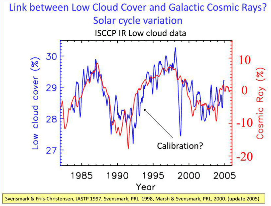
13. From 1996, Henrik Svensmark / Eigil Friis Christensen first show how cosmic rays control cloud cover.
    
    

14. The graph below is from a presentation in March 2018 by Henrik & Jacob Svensmark. It shows the strong connection over a 30 year period between cosmic ray variations, as modulated by the non-radiant features of solar activity [NRSA], and their effect on the level of cover from low clouds. This is able to explain NRSA's link with temperature on timescales of days to decades.

    This controlling role of the NRSA is crucial to the theory of the solar factor because major variation in total solar radiant heat output - RHO - is slow and therefore only able to account for climate changes on timescales from about 50 years upwards.

    

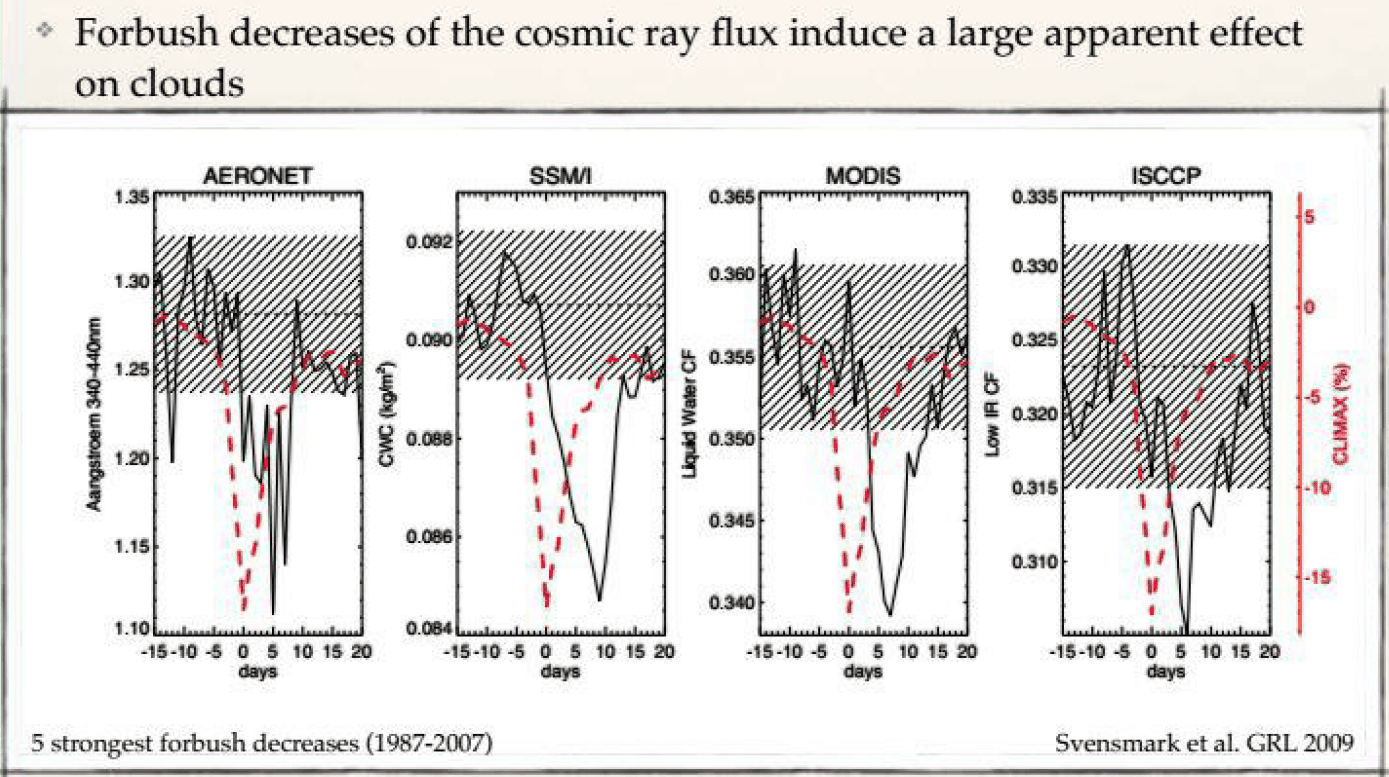
15. Clinching evidence for the link between variation in cosmic ray flux and the level of cloudiness comes from sudden and and short term decreases in this flux - known as Forbush decreases [see note below] - and their apparent effect on cloudiness within days, as shown by in the diagrams below

    

    Note on Forbush decreases. These arise from sudden and short term changes to the magnetic field of the solar plasma wind, which follow from ejections of material by the sun known as coronal mass ejecrions [CME's] - see Wikipedia for details

16. Rapid AMO warming from the mid 1990’s is covariant with:

    1. A decline in low cloud cover globally, leading to surface warming, and increased upper ocean heat content.
    2. Changes in the vertical distribution of water vapour: Declines in lower stratosphere water vapour leading to cooling. Increases in low-mid troposphere water vapour, at least due to higher SST’s coupled with an increase in surface wind speeds over the oceans, leading to low-mid troposphere warming.
    3. Reduced CO2 uptake in the warmer North Atlantic and in land regions made drier by the warm AMO phase (and increased El Nino).
       All because ocean phases vary inversely to changes in climate forcing.

17. Also see: The next Grand Solar Minimum, Cosmic Rays and Earth Changes (an introduction) BY SACHA DOBLER ON 14. JANUARY 2018

18. Strong coherance between Solar variability and the Monsoon in Oman between 9 and 6kyr. Neff et al, Nature 411 | 17 May 2001.
    
    Hat tip: Nir Shaviv
19. 
    
    
    
    Blue = C-14 proxy for solar activity
    Black = sea floor record for N Atlantic proxy for temperature
    Hat tip: Nir Shaviv, via this paper: Persistent Solar Influence on North Atlantic Climate During the Holocene, Bond et al, Science 294 | 7 Dec 2001
20. Shaviv: Correlation between the cosmic ray flux reconstruction (based on the exposure ages of Iron meteorites) and the geochemically reconstructed tropical temperature. The comparison between the two reconstructions reveals the dominant role of cosmic rays and the galactic “geography” as a climate driver over geological time scales. Figure 2 (below):
    

    The cosmic ray flux (Φ) and tropical temperature anomaly (ΔT) variations over the Phanerozoic. The upper curves describe the reconstructed CRF using iron meteorite exposure age data (Shaviv, 2002b). The blue line depicts the nominal CRF, while the yellow shading delineates the allowed error range. The two dashed curves are additional CRF reconstructions that fit within the acceptable range (together with the blue line, these three curves denote the three CRF reconstructions used in the model simulations). The red curve describes the nominal CRF reconstruction after its period was fine tuned to best fit the low-latitude temperature anomaly (i.e., it is the “blue” reconstruction, after the exact CRF periodicity was fine tuned, within the CRF reconstruction error). The bottom black curve depicts the 10/50 m.y. (see Fig. 1) smoothed temperature anomaly (ΔT) from Veizer et al. (2000). The red line is the predicted ΔT_model for the red curve above, taking into account also the secular long-term linear contribution (term B × t in equation 1). The green line is the residual. The largest residual is at 250 m.y. B.P., where only a few measurements of δ¹⁸O exist due to the dearth of fossils subsequent to the largest extinction event in Earth history. The top blue bars are as in Figure 1.
    
    Shaviv & Vezier 2003. "Celestial driver of Phanerozoic climate?" GSA Today 13(7):4-10 (2003). DOI: 10.1130/1052-5173(2003)013<0004:CDOPC>2.0.CO;2

21. Correlation between sea levels with solar cycles:
22. 300 years of Chinese spruce compared with sunspot counts averaged over the solar cycle length (blue).
    Hat tip Rog Tallbloke
    
23. Precipitation Climate and Solar modulation of the last 1000 years.Blue: Reconstructed Temperature Storch et al 2004, Red: solar modulation, after Muscheler et al 2007, Black: Reconstruction of precipitation amounts for the edge of the Tibetan Plateau. Sun & Liu (2012).
    
24. Global temperature anomaly is inversely proportional to specific humidity.
    
25. The sun controls the Mississippi, but there's a 34-year delay!
    
26. Both the East Asia Summer Monsoon and the Northern Australia Summer Monsoon retreated synchronously during the recent cold Little Ice Age in response to external forcings such as solar irradiance variation and possibly large volcanic eruptions. Fingerprints of the Sun on Asia-Australia Summer Monsoon Rainfalls during the Little Ice Age, Hong Yan, Willie Soon, & Bob Carter:
27. The following graph shows the recorded and predicted temperatures as plotted by Ole Humlum et al from their 2011 paper: “Identifying natural contributions to late Holocene climate change” (Elsevier); O. Humlum et al. / Global and Planetary Change 79 (2011 Central Greenland (GISP2) surface temperature of the past 4,000 years (blue line). Natural cycle modelled and forecasted data are shown by the green line. The coefficient of determination (r2) for the hindcasting period is 0.63.)

    “The causes of long (millennial scale) climate changes are generally poorly understood, and the issue is important for understanding the natural climate variability, as illustrated by ice and ocean cores. Also, the lack of a CO2 cycle at millennial time scales underscores the independence of such long climate variability from anthropogenic greenhouse enhancement.”

    “The warming following the Little Ice Age is generally perceived as a natural recovery from the previously cold period, and the effect of anthropogenic greenhouse enhancement is assumed to become important only after 1975 (IPCC, 2007). Our simple cyclic model (Fig.) is able to forecast the main features of this recorded warming until 2010, underlining that a significant part of the 20th century warming may be interpreted as the result of natural climatic variations, known to characterise at least the previous 4000 years.”

    

---

This blog began when I copied a comment by Ulric Lyons (listing 3 fingerprints of natural climate variability) from Judith Curries blog. | March 4, 2019 at 9:45 am. I expanded it by adding more fingerprints.

A climate fingerprint can be recognized as a relationship (correlation) between two, or more, variables. When these two things change at the same time, on multiple occasions, in the same, or opposite directions then we have an excellent 'fingerprint'.

IMHO, fingerprints and lack of them where they're expected are the best, and simplest, climate evidence. Because fingerprints are simple and obvious evidence. We can all understand them and most likely agree on them when the data and statistics are honest. When found in nature, fingerprints can be used as evidence in both validation and falsification of hypotheses.

I searched for 'fingerprint' at WUWT. Most of the articles here are about fingerprint claims made, or expected fingerprints not found. I think we should balance that with fingerprints actually found. We should put more emphasis on showing what the science IS, rather than just commenting on what other people think the fake science is, and why they are wrong.